Arithmetic–geometric mean

In mathematics, the arithmetic–geometric mean (AGM or agM) of two positive real numbers x and y is the mutual limit of a sequence of arithmetic means and a sequence of geometric means. The arithmetic–geometric mean is used in fast algorithms for exponential, trigonometric functions, and other special functions, as well as some mathematical constants, in particular, computing π.

The AGM is defined as the limit of the interdependent sequences ${\displaystyle a_{i}}$ and ${\displaystyle g_{i}}$. Assuming ${\displaystyle x\geq y\geq 0}$, we write:$${\displaystyle {\begin{aligned}a_{0}&=x,\\g_{0}&=y\\a_{n 1}&={\tfrac {1}{2}}(a_{n} g_{n}),\\g_{n 1}&={\sqrt {a_{n}g_{n}}}\,.\end{aligned}}}$$These two sequences converge to the same number, the arithmetic–geometric mean of x and y; it is denoted by M(x, y), or sometimes by agm(x, y) or AGM(x, y).

The arithmetic–geometric mean can be extended to complex numbers and, when the branches of the square root are allowed to be taken inconsistently, it is a multivalued function.

Example

To find the arithmetic–geometric mean of a₀ = 24 and g₀ = 6, iterate as follows:$${\displaystyle {\begin{array}{rcccl}a_{1}&=&{\tfrac {1}{2}}(24 6)&=&15\\g_{1}&=&{\sqrt {24\cdot 6}}&=&12\\a_{2}&=&{\tfrac {1}{2}}(15 12)&=&13.5\\g_{2}&=&{\sqrt {15\cdot 12}}&=&13.416\ 407\ 8649\dots \\&&\vdots &&\end{array}}}$$The first five iterations give the following values:

The number of digits in which a_n and g_n agree (underlined) approximately doubles with each iteration. The arithmetic–geometric mean of 24 and 6 is the common limit of these two sequences, which is approximately 13.4581714817256154207668131569743992430538388544.

History

The first algorithm based on this sequence pair appeared in the works of Lagrange. Its properties were further analyzed by Gauss.

Properties

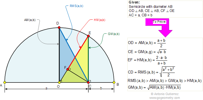
Both the geometric mean and arithmetic mean of two positive numbers x and y are between the two numbers. (They are strictly between when x ≠ y.) The geometric mean of two positive numbers is never greater than the arithmetic mean. So the geometric means are an increasing sequence g₀ ≤ g₁ ≤ g₂ ≤ ...; the arithmetic means are a decreasing sequence a₀ ≥ a₁ ≥ a₂ ≥ ...; and g_n ≤ M(x, y) ≤ a_n for any n. These are strict inequalities if x ≠ y.

M(x, y) is thus a number between x and y; it is also between the geometric and arithmetic mean of x and y.

If r ≥ 0 then M(rx, ry) = r M(x, y).

There is an integral-form expression for M(x, y):$${\displaystyle {\begin{aligned}M(x,y)&={\frac {\pi }{2}}\left(\int _{0}^{\frac {\pi }{2}}{\frac {d\theta }{\sqrt {x^{2}\cos ^{2}\theta y^{2}\sin ^{2}\theta }}}\right)^{-1}\\&=\pi \left(\int _{0}^{\infty }{\frac {dt}{\sqrt {t(t x^{2})(t y^{2})}}}\right)^{-1}\\&={\frac {\pi }{4}}\cdot {\frac {x y}{K\left({\frac {x-y}{x y}}\right)}}\end{aligned}}}$$where K(k) is the complete elliptic integral of the first kind:$${\displaystyle K(k)=\int _{0}^{\frac {\pi }{2}}{\frac {d\theta }{\sqrt {1-k^{2}\sin ^{2}\theta }}}}$$Since the arithmetic–geometric process converges so quickly, it provides an efficient way to compute elliptic integrals, which are used, for example, in elliptic filter design.

The arithmetic–geometric mean is connected to the Jacobi theta function ${\displaystyle \theta _{3}}$ by$${\displaystyle M(1,x)=\theta _{3}^{-2}\left(\exp \left(-\pi {\frac {M(1,x)}{M\left(1,{\sqrt {1-x^{2}}}\right)}}\right)\right)=\left(\sum _{n\in \mathbb {Z} }\exp \left(-n^{2}\pi {\frac {M(1,x)}{M\left(1,{\sqrt {1-x^{2}}}\right)}}\right)\right)^{-2},}$$which upon setting ${\displaystyle x=1/{\sqrt {2}}}$ gives$${\displaystyle M(1,1/{\sqrt {2}})=\left(\sum _{n\in \mathbb {Z} }e^{-n^{2}\pi }\right)^{-2}.}$$

Related concepts

The reciprocal of the arithmetic–geometric mean of 1 and the square root of 2 is Gauss's constant.$${\displaystyle {\frac {1}{M(1,{\sqrt {2}})}}=G=0.8346268\dots }$$In 1799, Gauss proved that$${\displaystyle M(1,{\sqrt {2}})={\frac {\pi }{\varpi }}}$$where ${\displaystyle \varpi }$ is the lemniscate constant.

In 1941, ${\displaystyle M(1,{\sqrt {2}})}$ (and hence ${\displaystyle G}$) was proved transcendental by Theodor Schneider. The set ${\displaystyle \{\pi ,M(1,1/{\sqrt {2}})\}}$ is algebraically independent over ${\displaystyle \mathbb {Q} }$, but the set ${\displaystyle \{\pi ,M(1,1/{\sqrt {2}}),M'(1,1/{\sqrt {2}})\}}$ (where the prime denotes the derivative with respect to the second variable) is not algebraically independent over ${\displaystyle \mathbb {Q} }$. In fact,$${\displaystyle \pi =2{\sqrt {2}}{\frac {M^{3}(1,1/{\sqrt {2}})}{M'(1,1/{\sqrt {2}})}}.}$$The geometric–harmonic mean GH can be calculated using analogous sequences of geometric and harmonic means, and in fact GH(x, y) = 1/M(1/x, 1/y) = xy/M(x, y). The arithmetic–harmonic mean is equivalent to the geometric mean.

The arithmetic–geometric mean can be used to compute – among others – logarithms, complete and incomplete elliptic integrals of the first and second kind, and Jacobi elliptic functions.

Proof of existence

The inequality of arithmetic and geometric means implies that$${\displaystyle g_{n}\leq a_{n}}$$and thus$${\displaystyle g_{n 1}={\sqrt {g_{n}\cdot a_{n}}}\geq {\sqrt {g_{n}\cdot g_{n}}}=g_{n}}$$that is, the sequence g_n is nondecreasing and bounded above by the larger of x and y. By the monotone convergence theorem, the sequence is convergent, so there exists a g such that:$${\displaystyle \lim _{n\to \infty }g_{n}=g}$$However, we can also see that:$${\displaystyle a_{n}={\frac {g_{n 1}^{2}}{g_{n}}}}$$ and so: $${\displaystyle \lim _{n\to \infty }a_{n}=\lim _{n\to \infty }{\frac {g_{n 1}^{2}}{g_{n}}}={\frac {g^{2}}{g}}=g}$$

Q.E.D.

Proof of the integral-form expression

This proof is given by Gauss. Let

$${\displaystyle I(x,y)=\int _{0}^{\pi /2}{\frac {d\theta }{\sqrt {x^{2}\cos ^{2}\theta y^{2}\sin ^{2}\theta }}},}$$

Changing the variable of integration to ${\displaystyle \theta '}$, where

$${\displaystyle \sin \theta ={\frac {2x\sin \theta '}{(x y) (x-y)\sin ^{2}\theta '}}\Rightarrow d(\sin \theta )=d\left({\frac {2x\sin \theta '}{(x y) (x-y)\sin ^{2}\theta '}}\right)\Rightarrow \cos \theta \ d\theta =2x{\frac {(x y)-(x-y)\sin ^{2}\theta '}{((x y) (x-y)\sin ^{2}\theta ')^{2}}}\ \cos \theta 'd\theta '}$$

$${\displaystyle \cos \theta ={\frac {\sqrt {(x y)^{2}-2(x^{2} y^{2})\sin ^{2}\theta ' (x-y)^{2}\sin ^{4}\theta '}}{(x y) (x-y)\sin ^{2}\theta '}}={\frac {\cos \theta '{\sqrt {(x-y)^{2}\cos ^{2}\theta ' 4xy}}}{(x y) (x-y)\sin ^{2}\theta '}}={\frac {\cos \theta '{\sqrt {(x y)^{2}\cos ^{2}\theta ' 4xy\sin ^{2}\theta '}}}{(x y) (x-y)\sin ^{2}\theta '}},}$$

$${\displaystyle \Rightarrow \cos \theta \ d\theta ={\frac {\cos \theta '{\sqrt {(x y)^{2}\cos ^{2}\theta ' 4xy\sin ^{2}\theta '}}}{(x y) (x-y)\sin ^{2}\theta '}}\ d\theta =2x{\frac {(x y)-(x-y)\sin ^{2}\theta '}{((x y) (x-y)\sin ^{2}\theta ')^{2}}}\ \cos \theta 'd\theta ',}$$

$${\displaystyle \Rightarrow d\theta ={\frac {x((x y)-(x-y)\sin ^{2}\theta ')}{((x y) (x-y)\sin ^{2}\theta ')}}{\frac {2d\theta '}{\sqrt {(x y)^{2}\cos ^{2}\theta ' 4xy\sin ^{2}\theta '}}}\ ,}$$ $${\displaystyle {\sqrt {x^{2}\cos ^{2}\theta y^{2}\sin ^{2}\theta }}={\frac {\sqrt {x^{2}((x y)^{2}-2(x^{2} y^{2})\sin ^{2}\theta ' (x-y)^{2}\sin ^{4}\theta ') 4x^{2}y^{2}\sin ^{2}\theta '}}{((x y) (x-y)\sin ^{2}\theta ')}}={\frac {x((x y)-(x-y)\sin ^{2}\theta ')}{((x y) (x-y)\sin ^{2}\theta ')}}}$$

This yields $${\displaystyle {\frac {d\theta }{\sqrt {x^{2}\cos ^{2}\theta y^{2}\sin ^{2}\theta }}}={\frac {2d\theta '}{\sqrt {(x y)^{2}\cos ^{2}\theta ' 4xy\sin ^{2}\theta '}}}={\frac {d\theta '}{\sqrt {(({\frac {x y}{2}})^{2}\cos ^{2}\theta ' ({\sqrt {xy}})^{2}\sin ^{2}\theta '}}},}$$

gives

$${\displaystyle {\begin{aligned}I(x,y)&=\int _{0}^{\pi /2}{\frac {d\theta '}{\sqrt {(({\frac {x y}{2}})^{2}\cos ^{2}\theta ' ({\sqrt {xy}})^{2}\sin ^{2}\theta '}}}\\&=I{\bigl (}{\tfrac {x y}{2}},{\sqrt {xy}}{\bigr )}.\end{aligned}}}$$

Thus, we have

$${\displaystyle {\begin{aligned}I(x,y)&=I(a_{1},g_{1})=I(a_{2},g_{2})=\cdots \\&=I{\bigl (}M(x,y),M(x,y){\bigr )}=\pi /{\bigr (}2M(x,y){\bigl )}.\end{aligned}}}$$ The last equality comes from observing that ${\displaystyle I(z,z)=\pi /(2z)}$.

Finally, we obtain the desired result

$${\displaystyle M(x,y)=\pi /{\bigl (}2I(x,y){\bigr )}.}$$

Applications

The number π

According to the Gauss–Legendre algorithm,

$${\displaystyle \pi ={\frac {4\,M(1,1/{\sqrt {2}})^{2}}{1-\displaystyle \sum _{j=1}^{\infty }2^{j 1}c_{j}^{2}}},}$$

where

$${\displaystyle c_{j}={\frac {1}{2}}\left(a_{j-1}-g_{j-1}\right),}$$

with ${\displaystyle a_{0}=1}$ and ${\displaystyle g_{0}=1/{\sqrt {2}}}$, which can be computed without loss of precision using

$${\displaystyle c_{j}={\frac {c_{j-1}^{2}}{4a_{j}}}.}$$

Complete elliptic integral K(sinα)

Taking ${\displaystyle a_{0}=1}$ and ${\displaystyle g_{0}=\cos \alpha }$ yields the AGM

$${\displaystyle M(1,\cos \alpha )={\frac {\pi }{2K(\sin \alpha )}},}$$

where K(k) is a complete elliptic integral of the first kind:

$${\displaystyle K(k)=\int _{0}^{\pi /2}(1-k^{2}\sin ^{2}\theta )^{-1/2}\,d\theta .}$$

That is to say that this quarter period may be efficiently computed through the AGM, $${\displaystyle K(k)={\frac {\pi }{2M(1,{\sqrt {1-k^{2}}})}}.}$$

Other applications

Using this property of the AGM along with the ascending transformations of John Landen, Richard P. Brent suggested the first AGM algorithms for the fast evaluation of elementary transcendental functions (e^x, cos x, sin x). Subsequently, many authors went on to study the use of the AGM algorithms.

See also

• Landen's transformation
• Gauss–Legendre algorithm
• Generalized mean

References

Notes

Citations

Sources